测序数据处理自用笔记

转录组数据处理笔记

一、前置环境

1.1 Linux子系统

首先肯定是在Linux上进行，我这边稍微记录一下现在装Linux子系统的步骤^[1]：

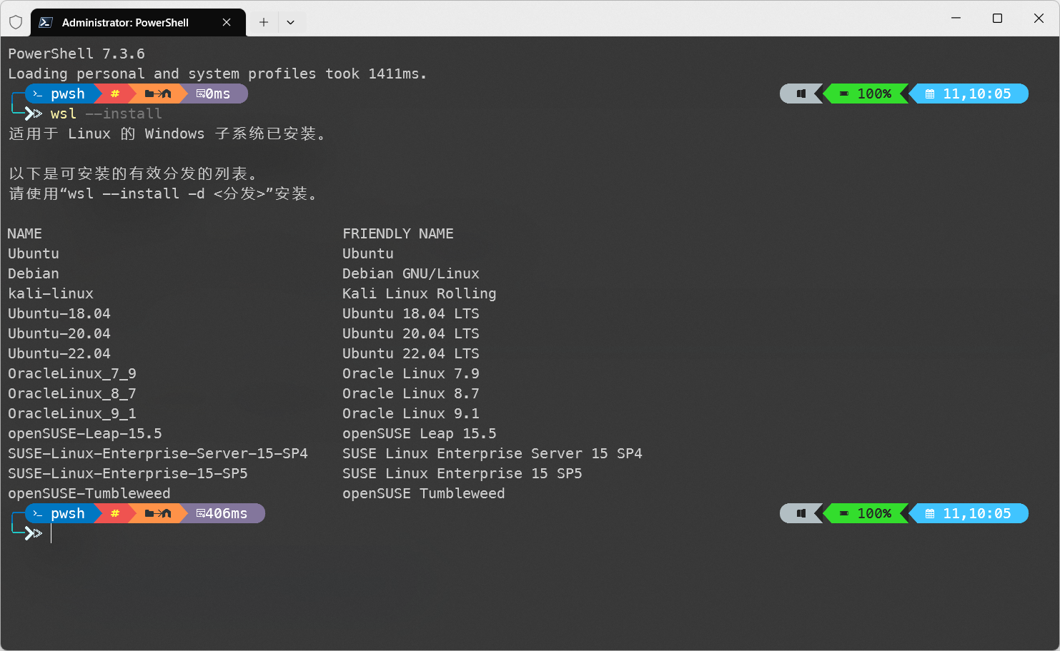
以管理员模式运行Windows terminal，并执行以下指令：

wsl --install

安装完毕后，再次运行此指令，能够看到如下界面：

wsl分支

接下来根据提示，安装指定的分支，例如我选择Ubuntu22：

wsl --install -d Ubuntu-22.04

运行期间会要求输入用户名密码等，跟着输入就行。

当使用完子系统之后，直接关闭窗口并不会结束子系统进程，这会导致其依然在系统内存中占用资源。

想要彻底关闭WSL，在power shell中执行以下指令：

wsl --shutdonn

1.2 conda安装及镜像配置

首先安装miniconda^[2]，下载安装脚本，并赋予其相应权限，之后运行脚本即可：

wget https://repo.anaconda.com/miniconda/Miniconda3-py310_23.5.2-0-Linux-x86_64.sh
sudo chmod 777 Miniconda3-py310_23.5.2-0-Linux-x86_64.sh
./Miniconda3-py310_23.5.2-0-Linux-x86_64.sh

具体文件名字视你下的版本而定

脚本运行期间，基本上是一路yes到底就行了。

conda安装完毕之后，重启系统或者通过一下指令刷新环境变量：

source .bashrc

接下来配置所使用的镜像^[3]，这里需要使用bioconda这个channel：

conda config --set show_channel_urls yes
nano .condarc

将配置文件修改如下：

channels:
  - defaults
show_channel_urls: true
default_channels:
  - https://mirrors.tuna.tsinghua.edu.cn/anaconda/pkgs/main
  - https://mirrors.tuna.tsinghua.edu.cn/anaconda/pkgs/r
  - https://mirrors.tuna.tsinghua.edu.cn/anaconda/pkgs/msys2
  - https://mirrors.tuna.tsinghua.edu.cn/anaconda/cloud/conda-forge
  - https://mirrors.tuna.tsinghua.edu.cn/anaconda/cloud/bioconda
custom_channels:
  conda-forge: https://mirrors.tuna.tsinghua.edu.cn/anaconda/cloud
  msys2: https://mirrors.tuna.tsinghua.edu.cn/anaconda/cloud
  bioconda: https://mirrors.tuna.tsinghua.edu.cn/anaconda/cloud
  menpo: https://mirrors.tuna.tsinghua.edu.cn/anaconda/cloud
  pytorch: https://mirrors.tuna.tsinghua.edu.cn/anaconda/cloud
  pytorch-lts: https://mirrors.tuna.tsinghua.edu.cn/anaconda/cloud
  simpleitk: https://mirrors.tuna.tsinghua.edu.cn/anaconda/cloud
  deepmodeling: https://mirrors.tuna.tsinghua.edu.cn/anaconda/cloud/

之后使用如下指令来清空缓存：

conda clean -i

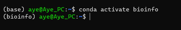
现在可以创建一个新的环境了：

conda create --name bioinfo python=3.10
conda activate bioinfo

二、质量分析

这里所使用到的软件为fastqc与multiqc，这俩其实用处差不多，只不过后者可以将多份数据进行整合。

2.1 软件安装

直接通过conda安装即可：

conda install fastqc multiqc

2.2 参数含义

FastQC^[4]

• -h 或 --help ：显示帮助信息
• -o <output_dir> 或 --outdir <output_dir>：指定输出目录，将生成的结果文件保存到指定的目录中
• -f <format> 或 --format <format>：指定输入文件的格式。常见的格式包括"fastq"、"bam"、"sam"等
• -t <threads> 或 --threads <threads>：指定线程数，用于加速分析。默认为1个线程
• -c <config_file> 或 --config <config_file>：指定配置文件，配置额外的参数等
• -k <kmersize> 或 --kmersize <kmersize>：指定用于检测存在的最大k-mer大小。默认为10
• -adapters <adapters_file>：指定adapter序列文件，用于adapter污染检测
• -limits <limits_file>：指定limits文件，用于制定可接受的范围，例如序列长度、GC含量等
• -extract：提取原始的FastQC zip文件，而不进行分析
• -q 或 --quiet：静默模式，只输出错误消息

MultiQC^[5]

• -h 或 --help ：显示帮助信息。
• -o <output_dir> 或 --outdir <output_dir>：指定输出目录，将生成的报告文件保存到指定的目录中。
• -c <config_file> 或 --config <config_file>：指定配置文件，自定义报告生成的规则和设置。
• -s 或 --fullnames：显示完整的样本名称，而不仅仅是文件名部分。
• --title <report_title>：指定报告的标题。
• -f 或 --force：强制重新生成报告，覆盖已存在的报告文件。
• --ignore <regexp>：忽略与指定正则表达式匹配的文件。
• --exclude <regexp>：排除与指定正则表达式匹配的文件。
• --no-ansi：禁用ANSI转义序列，不使用彩色输出。
• -q 或 --quiet：静默模式，只输出错误消息。

2.3 质量检测

由于这两个软件都无法自动创建目录，因此需要手动创建输出目录：

mkdir result

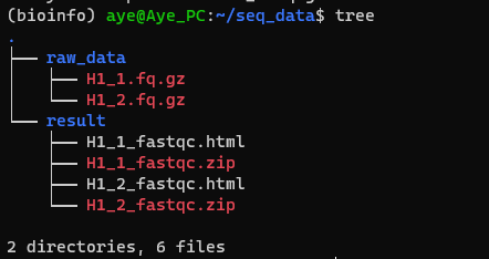
对于单个文件，使用fastqc进行分析，如：

fastqc -o result -f fastq -t 8 raw_data/H1_1.fq.gz

即可得到分析结果：

批量处理一个文件夹下的数据：

cd raw_data
ls *.gz |xargs fastqc -o ../result/ -t 8

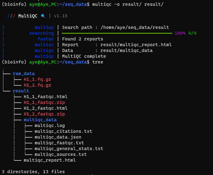
同时，可以使用MultiQC对多个数据文件进行整合：

multiqc -o result/ result/

三、数据清洗

3.1 软件安装

数据清洗使用的软件为Trim Galore和fastp，它前置依赖Cutadapt和FastQC

conda install cutadapt trim-galore fastp

3.2 参数含义

Trim Galore^[6]

• --quality：指定去除低质量reads的阈值，默认为20。 作用：去除质量低于指定阈值的reads
• --length：指定去除短reads的长度阈值，默认为20。 作用：去除长度低于指定阈值的reads
• --stringency：指定adapter剪切的严格程度，默认为1。 作用：调整adapter剪切的严格程度，值越高表示更严格的剪切
• --paired：指定输入的测序数据是否为配对的，默认为单端测序。 作用：指定处理的测序数据是否为配对的，以决定是否进行配对数据处理
• --phred33：：选择phred33或者phred64，表示测序平台使用的Phred quality score
• --fastqc：生成每个输入文件的质量评估报告，同时内部调用fastqc软件。 作用：生成测序数据的质量评估报告，以便进行质量控制
• --fastqc_args "<ARGS>" fastqc的参数
• --gzip：指定输出文件是否进行压缩，默认为否。 作用：选择是否对输出文件进行压缩，可以减小文件大小
• --cores：指定使用的CPU核心数，默认为1。 作用：指定trim-galore使用的CPU核心数，用于加速处理速度
• --output_dir：输入目录。需要提前建立目录，否则运行会报错

fastp^[7]

• -i, --in1：输入read1
• -o, --out1：输出read1
• -I, --in2：输入read2
• -O, --out2：输出read2
• -A, --disable_ adpter_ trimming：不过滤接头序列,默认过滤
• -f, --trim_ front1：去掉read1头部的几bp序列 ,默认为0
• -t, --trim _tail1：去掉read1尾部的几bp序列,默认为0
• -F, --trim_ front2：去掉read2头部的几bp序列,默认为0
• -T, --trim_ front2：去掉read2尾部的几bp序列,默认为0
• -q,--qualified_ quality_phred：质量值低于q的碱基将被过滤,默认为15
• -I, --length_ required：长度低于l的序列将被过滤,默认为15
• -n, --n_ base_ limit：序列中含N碱基多余n个将被过滤,默认为5
• -5,-3：开启滑窗质量裁剪
• -W：滑动窗口大小，默认4
• -M：滑窗裁剪平均质量，默认20
• -j, --json：生成可读的json文件
• -h, --html：生成html质控报告

3.3 清洗

使用Trim Galore

mkdir clean_data
mkdir clean_result

对于单个文件：

trim_galore --paired --cores 2 --phred33 --length 35 --stringency 1 --quality 25 --gzip --fastqc_args "-o trim_result/ -f fastq -t 8" --output_dir after_trim/ raw_data/H1_1.fq.gz raw_data/H1_2.fq.gz

批量处理：

mkdir clean_data
mkdir clean_result

ls raw_data/*_1.fq.gz > 1
ls raw_data/*_2.fq.gz > 2

paste 1 2 >config

cat config | while read id
  do
    arr=($id)
    fq1=${arr[0]}
    fq2=${arr[1]}
    trim_galore --paired --cores 2 --phred33 --length 35 --stringency 1 --quality 25 --gzip --fastqc_args "-o clean_result/ -f fastq -t 8" --output_dir clean_data/  $fq1 $fq2
  done

rm 1
rm 2
rm config

multiqc -o clean_result/ clean_result/

echo "done"

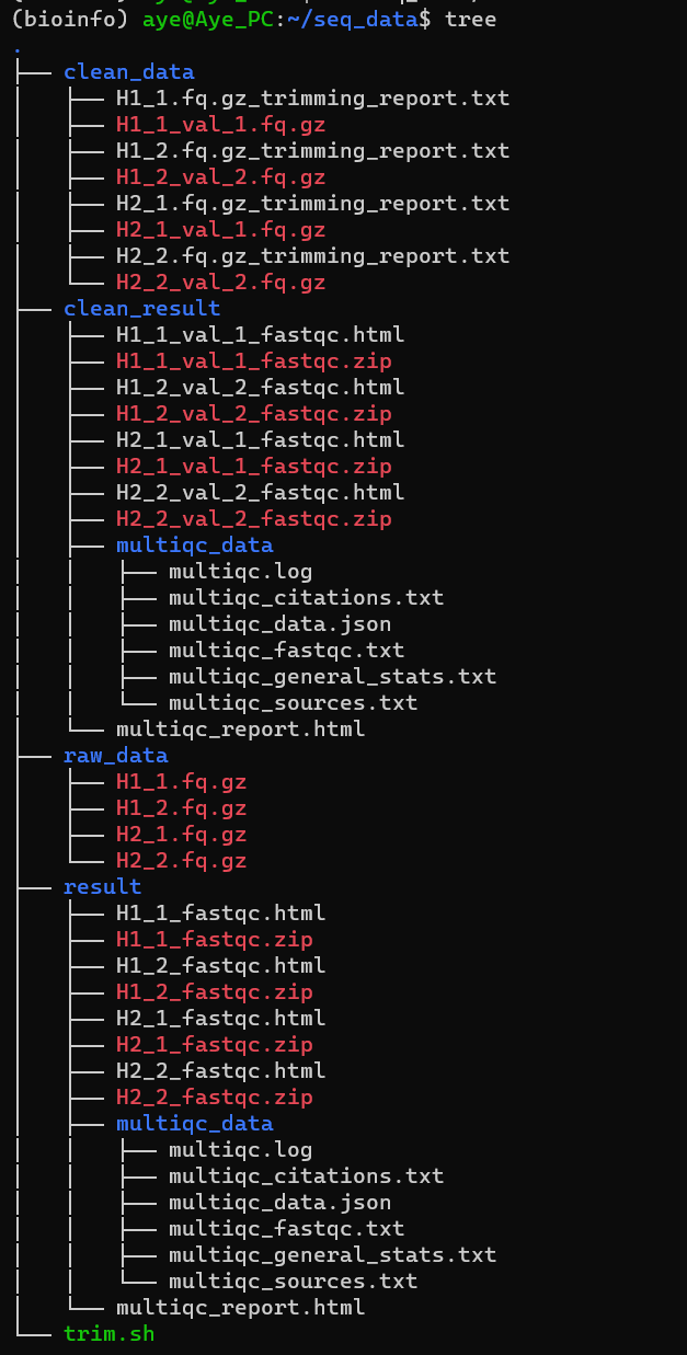
批处理执行完之后即可得到清洗后的数据和报告：

使用fastp

rm -rf clean_data clean_report

mkdir clean_data
mkdir clean_report

cd raw_data/
ls *_1.fq.gz > 1
ls *_2.fq.gz > 2

paste 1 2 >config

cat config | while read id
  do
    arr=($id)
    fq1=${arr[0]}
    fq2=${arr[1]}
    fq1_clean=$(echo "$fq1" | sed 's/.fq.gz/_clean.fq.gz/')
    fq2_clean=$(echo "$fq2" | sed 's/.fq.gz/_clean.fq.gz/')
    fastp -i $fq1 -o ../clean_data/$fq1_clean -I $fq2 -O ../clean_data/$fq2_clean -q 25 -l 35 --thread=8  -5 -3
  done

rm 1 2 config

cd ../clean_data
ls *_clean.fq.gz |xargs fastqc -o ../clean_report/ -t 8
cd ..
multiqc -o clean_report/ clean_report/

echo "done"

四、上游数据的比对计数

4.1 软件安装

hisat2

conda install hisat2 

samtools^[8]

sudo apt-get update
sudo apt-get install autoconf automake make gcc perl zlib1g-dev libbz2-dev liblzma-dev libcurl4-gnutls-dev libssl-dev libncurses5-dev

wget https://github.com/samtools/samtools/releases/download/1.18/samtools-1.18.tar.bz2
tar -xjvf samtools-1.18.tar.bz2
cd samtools-1.18
./configure
make
sudo make install

featureCounts

wget https://zenlayer.dl.sourceforge.net/project/subread/subread-2.0.6/subread-2.0.6-Linux-x86_64.tar.gz
tar -zxvf subread-2.0.6-Linux-x86_64.tar.gz
nano ~/.bashrc

在最下面添加一行：

export PATH="/home/aye/subread-2.0.6-Linux-x86_64/bin:$PATH"

使更改生效：

source ~/.bashrc

4.2 参数含义

hisat2

• -x：参考基因组索引文件的前缀。注意最后是/genome
• -1：双端测序结果的第一个文件。若有多组数据，使用逗号将文件分隔。Reads的长度可以不一致
• -2：双端测序结果的第二个文件。 若有多组数据，使用逗号将文件分隔，并且文件顺序要和-1参数对应。Reads的长度可以不一致
• -S：指定输出的SAM文件。
• -t：输出time
• -p：线程使用设置
• -U：单端数据文件。若有多组数据，使用逗号将文件分隔。可以和-1、 -2参数同时使用。 Reads的长度可以不一致
• --sra-acc：输入SRA登录号, 比如SRR353653, SRR353654。多组数据之间使用逗号分隔。HISAT将自动下载并识别数据类型，进行比对

samtools^[9]

• view：用于将sam文件转化为bam文件
  • -b：该参数设置输出 BAM 格式，默认下输出是 SAM 格式文件
  • -h：默认下输出的 sam 格式文件不带 header，该参数设定输出sam文件时带 header 信息
  • -H：仅仅输出文件的头文件
  • -S：默认下输入是 BAM 文件，若是输入是 SAM 文件，则最好加该参数，否则有时候会报错。
  • -u：该参数的使用需要有-b参数，能节约时间，但是需要更多磁盘空间。
  • -c：仅输出匹配的统计记录
  • -L：仅包括和bed文件存在overlap的reads
  • -o：输出文件的名称
  • -F：过滤flag，仅输出指定FLAG值的序列
  • -q：比对的最低质量值，一般认为20就为unique比对了，可以结合上述-bF参数使用使用提取特定的比对结果
  • -@：指使用的线程数
• sort：对bam文件进行排序
  • -n：设定排序方式按short reads的ID排序。默认下是按序列在fasta文件中的顺序（即header）和序列从左往右的位点排序。
  • -m INT：设置每个线程的最大内存，单位可以是K/M/G，默认是 768M。对于处理大数据时，如果内存够用，则设置大点的值，以节约时间。
  • -t TAG：按照TAG值排序
  • -o FILE：输出到文件中，加文件名
• index：建立索引，并生成bai文件
• flagstat：输出比对统计结果
  • -@：指使用的线程数

featureCounts^[10]

• -a：指定注释文件

• -o：指定输出文件

• -p：设置此参数后，使用fragments (或 templates)代替reads计数。只对paired-end reads有效

• -t：指定GTF注释文件中的feature类型。默认：exon

  • exon：外显子，基因组中包含的编码序列片段。

  • CDS (Coding Sequence)：编码序列，用于描述外显子中编码蛋白质的部分。

  • start_codon：起始密码子，表示编码蛋白质的起始位置。

  • stop_codon：终止密码子，表示编码蛋白质的终止位置。

  • UTR (Untranslated Region)：未翻译区域，编码序列中没有被翻译为蛋白质的区域。

  • transcript：转录本，表示基因的一个转录过程，包含一系列的外显子。

  • gene：基因，包含一个或多个转录本。

  • tRNA：转移RNA，一类用于将氨基酸传递到翻译中的蛋白质合成过程的分子。

  • rRNA：核糖体RNA，一类参与蛋白质合成的RNA分子。

  • snoRNA：小核仁RNA，参与核仁中的RNA加工和修饰。

  • miRNA：微RNA，一类通过调控基因表达参与调节细胞内RNA稳定性的小分子RNA。

  • snRNA：小核RNA，参与剪接反应和转录调控。

• -g：指定GTF注释文件中属性的类型。默认：gene_id

  • gene_id：基因的唯一标识符。

  • transcript_id：转录本的唯一标识符。

  • gene_name：基因的名称。

  • transcript_name：转录本的名称。

  • exon_number：外显子的编号。

  • exon_id：外显子的唯一标识符。

  • protein_id：蛋白质序列的唯一标识符。

  • gene_biotype：基因的生物类型，例如编码蛋白质的基因、非编码RNA基因等。

  • transcript_biotype：转录本的生物类型，例如编码蛋白质的转录本、非编码RNA转录本等。

  • gene_source：基因注释来源，表示该基因的来源数据库或参考序列。

  • transcript_source：转录本注释来源，表示该转录本的来源数据库或参考序列。

  • gene_symbol：基因的符号名称。

  • transcript_symbol：转录本的符号名称。

• -f：在feature水平计数 (如对外显子计数)

• -O：统计所有重叠的的meta-features的reads

• -C：对于比对到不同染色体或相同染色体的不同链的read对，不进行计数

• -T：使用线程

4.3 数据处理

get sam file

首先使用hisat2比对基因组得到sam文件，这里需要先下载参考基因组，因为我这里用的是人类细胞，所以使用hg38：

cd
mkdir -p reference/index/hisat
cd reference/index/hisat/
wget https://genome-idx.s3.amazonaws.com/hisat/hg38_genome.tar.gz
tar -zxvf hg38_genome.tar.gz

这玩意很大，下不下来也可以考虑使用别的方法下载后上传到服务器

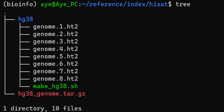
下载并解压后文件如下：

接下来比对基因组

hisat2 --dta -t -x ../../reference/index/hisat/hg38/genome -1 H1_1_clean.fq.gz -2 H1_2_clean.fq.gz -p 4 -S hisat2_hg38data/H1.sam

这里genome是参考基因组文件的前缀

sam to bam

之后，使用samtools进行进一步操作，首先是将sam文件转化为bam文件：

samtools view -@ 8 -bS -o hisat2_hg38data/H1_1.bam hisat2_hg38data/H1_1.sam

sort and index

接下来对bam进行排序:

samtools sort -@ 8 -o hisat2_hg38data/H1_1.sort.bam hisat2_hg38data/H1_1.bam

之后对使用排序好的文件建立索引

samtools index hisat2_hg38data/H1_1.sort.bam

最后，将比对结果输入到文件中保存：

samtools flagstat -@ 8 -O json hisat2_hg38data/H1_1.sort.bam > hisat2_hg38data/H1_1.sort.flagsata

count table

使用featureCounts获得counts.txt：

featureCounts -a ../reference/gtf/Homo_sapiens.GRCh38.110.chr.gtf.gz -g gene_id -t gene -O -p -T 8 -C -o counts/counts.txt hisat2_hg38data/*.sort.bam

批量处理：

rm -rf hisat2_hg38data/
mkdir hisat2_hg38data

cd clean_data/
ls *1_clean.fq.gz > 1
ls *2_clean.fq.gz > 2
paste 1 2 >config

cat config | while read id
  do
    arr=($id)
    fq1=${arr[0]}
    fq2=${arr[1]}
    output=$(echo "$fq1" | sed 's/_1_clean.fq.gz/.sam/')
    echo "hisat2 --dta -t -x ../../reference/index/hisat/hg38/genome -1 $fq1 -2 $fq2 -p 8 -S ../hisat2_hg38data/$output"
    hisat2 --dta -t -x ../../reference/index/hisat/hg38/genome -1 $fq1 -2 $fq2 -p 8 -S ../hisat2_hg38data/$output
  done
  
rm 1 2 config

cd ../hisat2_hg38data

echo "start sam to bam and sorting..."
ls *.sam | xargs -I {} sh -c 'samtools view -@ 8 -bS {} | samtools sort -@ 8 -o $(basename {} .sam).sort.bam'
echo "done, removing sam file..."
ls *.sam | xargs rm
echo "done"
tree

echo "start indexing..."
ls *.sort.bam | xargs samtools index -M 
echo "done"

echo "saving to flagsata..."
ls *.sort.bam | xargs -I {} sh -c 'samtools flagstat -@ 8 {} > $(basename {} .bam).flagstat'
echo "done"

multiqc ./

cd ..
rm -rf counts
mkdir counts

featureCounts -a ../reference/gtf/Homo_sapiens.GRCh38.110.chr.gtf.gz -g gene_id -t gene -O -p -T 8 -C -o counts/counts.txt hisat2_hg38data/*.sort.bam

4.4 结果解读^[11]

hisat2

19429766 reads; of these: # reads总数
  19429766 (100.00%) were paired; of these: # 配对的reads数量
    1066192 (5.49%) aligned concordantly 0 times # 一致地比对了0次的reads数量
    14853850 (76.45%) aligned concordantly exactly 1 time # 一致地比对了1次的reads数量
    3509724 (18.06%) aligned concordantly >1 times # 一致地比对了大于1次的reads数量
    ----
    1066192 pairs aligned concordantly 0 times; of these: # 一致地比对了0次的reads数量中：
      54954 (5.15%) aligned discordantly 1 time # 不一致地比对了1次的reads数量
    ----
    1011238 pairs aligned 0 times concordantly or discordantly; of these: #一致或不一致地比对了0次的reads数量中：
      2022476 mates make up the pairs; of these: # 配对的reads数量中：
        1211647 (59.91%) aligned 0 times #比对0次的数量
        607196 (30.02%) aligned exactly 1 time #比对1次的数量
        203633 (10.07%) aligned >1 times #比对大于1次的数量
96.88% overall alignment rate # mapping rate，由mapped reads number/total reads number的比例计算得到
[bam_sort_core] merging from 20 files and 4 in-memory blocks...

samtools

51231959 + 0 in total (QC-passed reads + QC-failed reads) #共有51231959条reads通过QC+0条reads未通过QC，后面的信息行中+后的都是代表QC没通过的reads的数量。
12372427 + 0 secondary
0 + 0 supplementary
0 + 0 duplicates
50020312 + 0 mapped (97.63% : N/A) # 97.63%比例的reads mapping到参考序列上，这就是mapping record rate
38859532 + 0 paired in sequencing
19429766 + 0 read1 # 双端reads中read1的总数
19429766 + 0 read2 # 双端reads中read2的总数
36727148 + 0 properly paired (94.51% : N/A) # 94.51%比例的reads成对的映射上
37160066 + 0 with itself and mate mapped # read映射上但配对read没映射上的数量
487819 + 0 singletons (1.26% : N/A) # 1.26%比例的read没映射上的同时，配对read映射上了
289948 + 0 with mate mapped to a different chr # reads和配对reads映射到不同染色体的情况下的reads数量
205767 + 0 with mate mapped to a different chr (mapQ>=5) # reads和配对reads映射到不同染色体，且映射质量大于等于5的情况下的reads数量

五、表达水平计算

经由上一步，得到了counts.txt，接下来就基于它进行进一步的计算。

虽然主流都是R语言，不过我比较属性python，反正都是大数据处理，没差别（

5.1 count的结构

我这里根据上面的参数，生成的count结构如下所示：

• Geneid：基因的唯一标识符
• Chr：基因所在的染色体
• Start：基因在染色体上的起始位置
• End：基因在染色体上的终止位置
• Strand：基因在染色体上的定向，正义链为"+", 反义链为"-"
• Length：基因的长度，单位为碱基
• H1、H2：基因在样品中的表达量

5.2 RPKM、FPKM和TPM^[12]

计算步骤

RPKM和FPKM计算方法一致，区别仅在于原始数据是否使用双端测序得来，其公式为：

\[ \begin{align} RPKM(x) &= \frac{Reads\ per\ transcription}{\frac{totla\ reads}{10^6} \times \frac{transcription\ length}{1000}}\\ &= \frac{10^9 \times C_x}{R \times L_x} \end{align} \]

具体而言，可以分成三步：

1. 对read count求和，并除以1000000
2. 将每一个read count除以上面的结果，得到RPM（read per million）
3. 将RPM除以length再乘以1000，得到RPKM

TPM类似，其计算公式为：

\[ TPM(X)=\frac{C_x \times r \times 10^6}{L_x \times T} \]

具体步骤也可以分为三步：

1. 将每一个read count除以length，乘以1000，得到RPK
2. 对RPK求和并除以1000000
3. 再用RPK除以上面的结果，得到TPM

程序

import pandas as pd
import matplotlib.pyplot as plt
import numpy as np

counts_df = pd.read_csv('counts.txt', sep='\t')

print(counts_df.columns)

express_num = len(counts_df) - 1
print(f'表达的基因数为:{express_num}')

count_10 = ((counts_df['H1'] > 10) | (counts_df['H2'] > 10)).sum()
print(f"有{count_10}个基因read count > 10。")

# FPKM
FPKM = pd.DataFrame()
FPKM['Geneid'] = counts_df['Geneid']

FMP1 = counts_df['H1'] / (counts_df['H1'].sum() / 10 ** 9)
FMP2 = counts_df['H2'] / (counts_df['H2'].sum() / 10 ** 9)

FPKM['H1'] = (FMP1 / counts_df['Length']) * 10 ** 3
FPKM['H2'] = (FMP2 / counts_df['Length']) * 10 ** 3

FPKM.to_csv('fpkm.csv', sep='\t', index=False)

# TPM
TPM = pd.DataFrame()
TPM['Geneid'] = counts_df['Geneid']

RPK1 = (counts_df['H1'] / counts_df['Length']) * 10 ** 3
RPK2 = (counts_df['H2'] / counts_df['Length']) * 10 ** 3

TPM['H1'] = RPK1 / (sum(RPK1) / 10 ** 6)
TPM['H2'] = RPK2 / (sum(RPK2) / 10 ** 6)

TPM.to_csv('tpm.csv', sep='\t', index=False)

# plot
data_1 = {'H1': np.log2(FPKM['H1'] + 1),
          'H2': np.log2(FPKM['H2'] + 1)}
FPKM_COPY = pd.DataFrame(data_1)
FPKM_COPY = FPKM_COPY.replace(0, np.nan)

FPKM_COPY.plot(kind='density')
plt.legend()
plt.xlabel('log2(FPKM+1)')
plt.ylabel('Density')
plt.title('Density of FPKM')
plt.show()

data_2 = {'H1': np.log2(TPM['H1'] + 1),
          'H2': np.log2(TPM['H2'] + 1)}
TPM_COPY = pd.DataFrame(data_2)
TPM_COPY = TPM_COPY.replace(0, np.nan)

TPM_COPY.plot(kind='density')
plt.legend()
plt.xlabel('log2(TPM+1)')
plt.ylabel('Density')
plt.title('Density of TPM')
plt.show()

print('done')

参考

1. https://learn.microsoft.com/en-us/windows/wsl/install ↩︎
2. https://conda.io/projects/conda/en/stable/user-guide/install/index.html ↩︎
3. https://mirrors.tuna.tsinghua.edu.cn/help/anaconda/ ↩︎
4. https://github.com/s-andrews/FastQC ↩︎
5. https://multiqc.info/ ↩︎
6. https://github.com/FelixKrueger/TrimGalore ↩︎
7. https://github.com/OpenGene/fastp ↩︎
8. https://github.com/samtools/samtools/blob/develop/INSTALL ↩︎
9. samtools的安装和使用 ↩︎
10. https://zh.wikibooks.org/wiki/生物信息学/featureCounts ↩︎
11. 基因组质量评估:(五)mapping法：2.samtools计算mapping rate ↩︎
12. P25 25.RPKM FPKM and TPM Clearly Explained ↩︎
13. 文件格式01：GTF与GFF文件 ↩︎